How to Tell Someone’s Age When All You Know Is Her Name
Emily Kothe
2018-12-01
Source:vignettes/guess_the_age.Rmd
guess_the_age.RmdThis vignette is based on this FiveThirtyEight article How to Tell Someone’s Age When All You Know Is Her Name. That article demonstrated how you could use actuarial life tables and a database of baby names to estimate the age of living Americans with a given name.
In this vignette we use the nzbabynames data set and the NZ complete cohort actuarial life tables to calculate the median age of individuals with a given first name.1.
An “old” name
Let’s start with one name that is sterotypically ‘old’ - Ethel
library(ggplot2)
library(matrixStats)
library(dplyr)
library(nzbabynames)
library(stringr)
library(lubridate)

name_of_interest <- "Ethel"

df <- life_tables %>%
  filter(percentile == "median") %>%
  filter(age == (lubridate::year(Sys.Date()) - yearofbirth)) %>%
  mutate(prop_still_alive = lx/100000,
         Year = yearofbirth,
         Sex = stringr::str_to_title(sex)) %>%
  right_join(filter(nzbabynames, Name == name_of_interest), by= c("Year", "Sex")) %>%
  mutate(prop_still_alive = case_when(
    Year < 1918 ~ 0,
    TRUE ~ prop_still_alive),
  Name = case_when(
    is.na(Name) ~ name_of_interest,
    TRUE ~ Name),
  Count = case_when(
    is.na(Count) ~ 0,
    TRUE ~ as.numeric(Count)),
  alive_count = Count * prop_still_alive)

med_age <- df %>%
  summarise(wted_median = weightedMedian(age, w = alive_count, na.rm = TRUE))

max <- max(df$Count)

peak <- df %>%
  filter(Count == max)

ggplot(data = df, aes(x = Year)) +
  geom_col(aes(y = Count), fill="grey")+
  geom_col(aes(y = alive_count), fill="cornflowerblue") +
  scale_x_continuous(limits = c(1900, 2016)) +
  coord_cartesian(expand = FALSE) +
  theme_classic()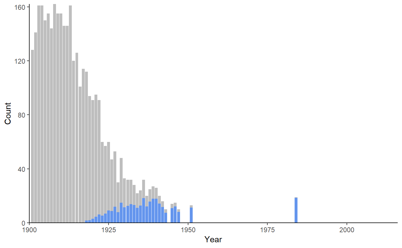
Ethel peaked in 1908 when 162 Ethels were born. Based on the actuarial data, 9% of Ethels born between 1900 and 2017 would still be alive in 2018. The median age of an Ethel still alive, would be 82 years.
And a young one
Let’s contrast that with a ‘younger’ name - Brittany.
name_of_interest <- "Brittany"

df <- life_tables %>%
  filter(percentile == "median") %>%
  filter(age == (lubridate::year(Sys.Date()) - yearofbirth)) %>%
  mutate(prop_still_alive = lx/100000,
         Year = yearofbirth,
         Sex = stringr::str_to_title(sex)) %>%
  right_join(filter(nzbabynames, Name == name_of_interest), by= c("Year", "Sex")) %>%
  mutate(prop_still_alive = case_when(
    Year < 1918 ~ 0,
    TRUE ~ prop_still_alive),
  Name = case_when(
    is.na(Name) ~ name_of_interest,
    TRUE ~ Name),
  Count = case_when(
    is.na(Count) ~ 0,
    TRUE ~ as.numeric(Count)),
  alive_count = Count * prop_still_alive)

med_age <- df %>%
  summarise(wted_median = weightedMedian(age, w = alive_count, na.rm = TRUE))

max <- max(df$Count)

peak <- df %>%
  filter(Count == max)

ggplot(data = df, aes(x = Year)) +
  geom_col(aes(y = Count), fill="grey")+
  geom_col(aes(y = alive_count), fill="cornflowerblue") +
  scale_x_continuous(limits = c(1900, 2016)) +
  coord_cartesian(expand = FALSE) +
  theme_classic()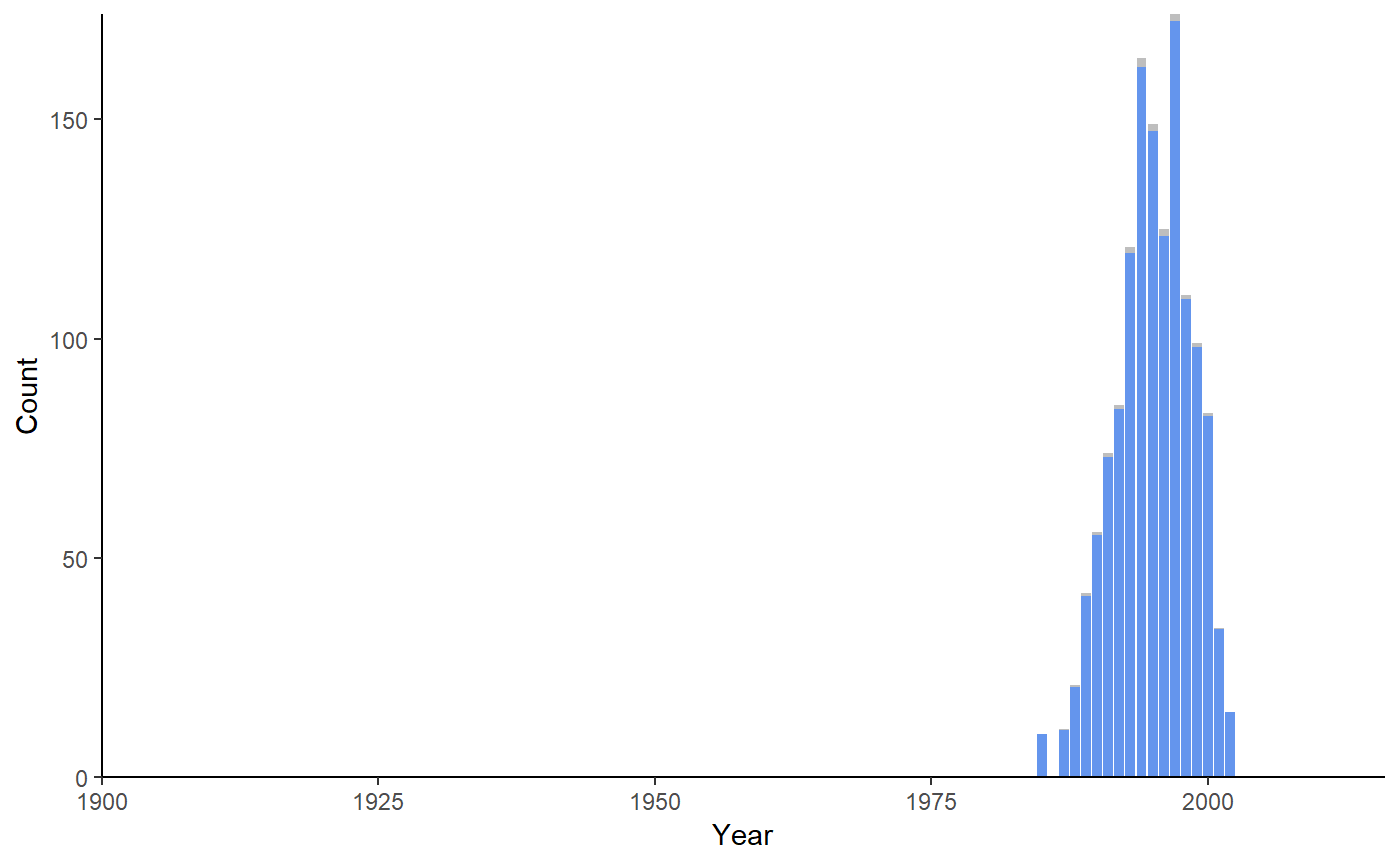
Brittany peaked in 1997 when 174 Brittanys were born. Based on the actuarial data, 99% of Brittanys born between 1900 and 2017 would still be alive in 2018. The median age of an Brittany still alive, would be 23 years.
Finally a less informative name
Ethel and Brittany are both names with pretty clear trajectories. But of course some names rise and fall over time. Let’s pick one of these - Joseph
name_of_interest <- "Joseph"

df <- life_tables %>%
  filter(percentile == "median") %>%
  filter(age == (lubridate::year(Sys.Date()) - yearofbirth)) %>%
  mutate(prop_still_alive = lx/100000,
         Year = yearofbirth,
         Sex = stringr::str_to_title(sex)) %>%
  right_join(filter(nzbabynames, Name == name_of_interest), by= c("Year", "Sex")) %>%
  mutate(prop_still_alive = case_when(
    Year < 1918 ~ 0,
    TRUE ~ prop_still_alive),
  Name = case_when(
    is.na(Name) ~ name_of_interest,
    TRUE ~ Name),
  Count = case_when(
    is.na(Count) ~ 0,
    TRUE ~ as.numeric(Count)),
  alive_count = Count * prop_still_alive)

med_age <- df %>%
  summarise(wted_median = weightedMedian(age, w = alive_count, na.rm = TRUE))

max <- max(df$Count)

peak <- df %>%
  filter(Count == max)

ggplot(data = df, aes(x = Year)) +
  geom_col(aes(y = Count), fill="grey")+
  geom_col(aes(y = alive_count), fill="cornflowerblue") +
  scale_x_continuous(limits = c(1900, 2016)) +
  coord_cartesian(expand = FALSE) +
  theme_classic()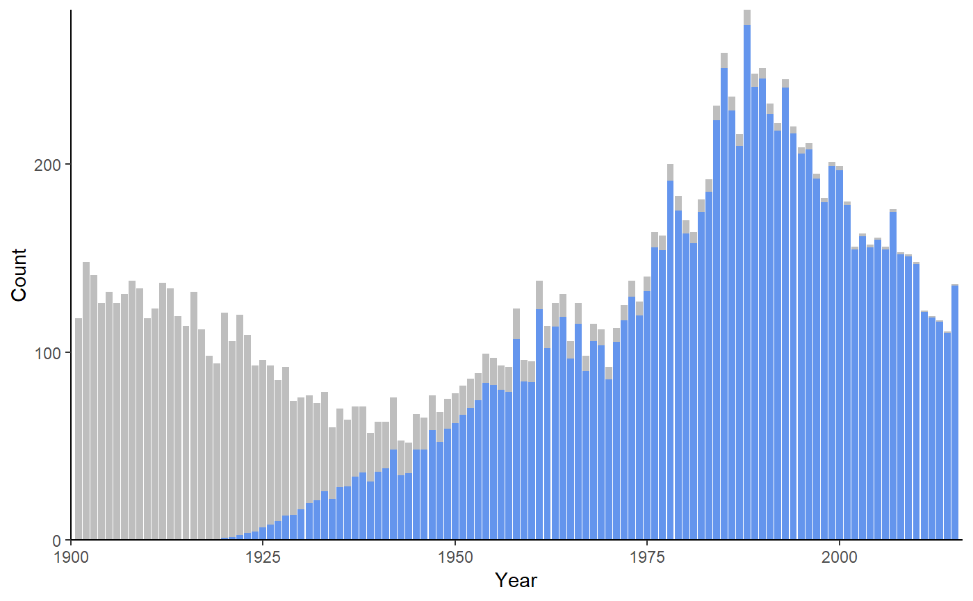
Joseph peaked in 1988 when 282 Josephs were born. Based on the actuarial data, 70% of Josephs born between 1900 and 2017 would still be alive in 2018. The median age of an Joseph still alive, would be 32 years.
However, note that while there is a clear peak in 1988 this name has had much more consistent consistent staying power than either Ethel or Brittany, meaning that you might be less confident about guessing the age of any given Joseph based on name alone. Put more formally, the interquartile range (and thus uncertainty) around the estimated age for Joseph is much greater than around Ethel or Brittany.
Like FiveThirtyEight we assume that people of the same sex die at the same rate regardless of their name - in practice will vary by a number of factors related to both name and life expectancy such as ethnicity↩