Top 10 Names

One popular way to understand baby names is to look at the most popular names in any given year.

Here let’s look at the Top 10 names for each year in our data set.

Start by reading in the data and creating a rank for each name by Sex and Year.

library(nzbabynames)
library(dplyr)
#> 
#> Attaching package: 'dplyr'
#> The following objects are masked from 'package:stats':
#> 
#>     filter, lag
#> The following objects are masked from 'package:base':
#> 
#>     intersect, setdiff, setequal, union


names <- nzbabynames

names <- names %>% 
  group_by(Sex, Year) %>% 
  arrange(-Count) %>% 
  mutate(Rank = seq_along(Count))

names
#> # A tibble: 66,653 x 5
#> # Groups:   Sex, Year [236]
#>     Year Sex   Name  Count  Rank
#>    <int> <chr> <chr> <int> <int>
#>  1  1947 Male  John   1628     1
#>  2  1948 Male  John   1575     1
#>  3  1946 Male  John   1561     1
#>  4  1963 Male  David  1513     1
#>  5  1949 Male  John   1504     1
#>  6  1958 Male  Peter  1484     1
#>  7  1962 Male  David  1478     1
#>  8  1956 Male  Peter  1451     1
#>  9  1957 Male  Peter  1431     1
#> 10  1950 Male  John   1403     1
#> # ... with 66,643 more rows

Now let’s filter the data set so we only have names in the Top 10 in any given year

names_top <- names %>%
  filter(Rank <= 10) 

tail(names_top)
#> # A tibble: 6 x 5
#> # Groups:   Sex, Year [5]
#>    Year Sex    Name      Count  Rank
#>   <int> <chr>  <chr>     <int> <int>
#> 1  1934 Female Jean        175    10
#> 2  1903 Female Elizabeth   173    10
#> 3  1901 Female Doris       172     9
#> 4  1919 Female Eileen      166    10
#> 5  1900 Female Elsie       166    10
#> 6  1901 Female Florence    165    10

We can find the most popular names in a given year

names_top %>% 
  filter(Year == 1985, Rank == 1)
#> # A tibble: 2 x 5
#> # Groups:   Sex, Year [2]
#>    Year Sex    Name   Count  Rank
#>   <int> <chr>  <chr>  <int> <int>
#> 1  1985 Male   Daniel   755     1
#> 2  1985 Female Sarah    657     1

I could also plot names over time. Here I’ll use ggplot2 and gganimate to plot male and female names separately so it’s easier to read.

library(ggplot2)
library(gganimate)

names_top_female <- names_top %>%
  filter(Sex == "Female") 

time <- ggplot(names_top_female, aes(x = Rank, y = Count, fill = Name)) +
  geom_col() + 
  facet_wrap("Sex") +
  geom_text(aes(label = Name), vjust = -0.5, size = 3) +
  theme_classic() +
  theme(legend.position="none") +
  labs(title="{current_frame}") +
  transition_manual(Year)

animate(time, duration=120)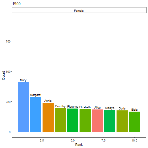

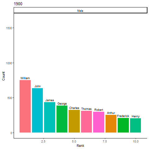
library(ggplot2)
library(gganimate)

names_top_male <- names_top %>%
  filter(Sex == "Male") 

time <- ggplot(names_top_male, aes(x = Rank, y = Count, fill = Name)) +
  geom_col() + 
  facet_wrap("Sex") +
  geom_text(aes(label = Name), vjust = -0.5, size = 3) +
  theme_classic() +
  theme(legend.position="none") +
  labs(title="{current_frame}") +
  transition_manual(Year)

animate(time, duration=120)

Emily Kothe

2018-12-01